[Review] Direct Sparse Odometry(DSO) (Eng)

Introduction

Pre-requisites for understanding DSO:

• micro knowledge about Lie Algebra

I will skip miscs about

• Direct vs Indirect
• Dense vs Sparse
• Mono vs Stereo

you can always refer the original paper for the details.

Remarks of DSO

Sparse Direct Mononular Visual Odometry

Jointly optimize model parameters including camera poses, camera intrinsics, geometry parameters - inverse depth.

Sliding window optimization, marginalizing on

• Old camera poses
• Points that leaves FOV

which is inspired by [1]

Utilizing full advantages of photometric calibration

• Lens attenuation
• Gamma correction
• Known exposure times

In conclusion, DSO is ...

optimization of the photometric error from monocular camera over a sliding window, taking into account a photometric calibrated model.

Direct Sparse Model

Notation

$$
\boxplus : se(3)\times SE(3) \rarr SE(3) \
x_i\boxplus T_i:=e^{\hat{x_i}}\cdot T_i
$$

Calibration

Geometric Camera Calibration

TBD

Photometric Camera Calibration

TBD

Model Formulation

Establishing photometric energy term

A photometric error of a point $p\in \Omega_i$ in reference frame $I_i$, observed in a target frame $I_j$, as the weighted sum of sqaured distance (SSD) over a 8 neighboring pixels, $N_{\bf p}$ (similar to first and second order irradiance derivatives of the center).

Energy equation depends on:

• the point’s inverse depth $d_p$
• the camera intrinsics ${\bf c}$
• the poses of the involved frames $T_i, T_j$
• their brightness transfer function parameters $a_i, b_i, a_j, b_j.$

$$
E_{{\bf p}j}:=\sum_{{\bf p} \in N_{\bf p}}{w_p \bigg|\bigg| (I_j[{\bf p}']-b_j)-\frac{t_je^{a_j}}{t_ie^{a_i}}(I_i[{\bf p}]-b_i) \bigg|\bigg|_\gamma}
$$

where $t_i, t_j$ are exposure time of the images $I_i, I_j$, and $||\cdot||_\gamma$ the Huber norm.

What is Huber norm?

In short, Huber norm is a robust distance metric.

Gradient-dependent weighting down-weights high gradient pixels.
$$
w_p:=\frac{c^2}{c^2+|\nabla I_i({\bf p})|^2_2}
$$
Radical change around some point can induce large energy difference, so this weighting can marginalize small geometrical error.

affine brightness transfer function $e^{-a_i}(I_i-b_i)$

$a_i, b_i, a_j, b_j$ are coefficients to correct for affine illumination changes

Projected point position $p'$ in the host frame, with inverse depth $d_p$. 3D depth is represented as inverse depth in a reference frame and thus have one degree of freedom.

$$ {\bf p}'=\Pi_c(R\Pi_c^{-1}({\bf p},d_{\bf p})+t)\\ \begin{bmatrix} R & t \\ 0 & 1 \end{bmatrix}:=T_jT_i^{-1} $$

$\Pi_c$ is projection from $\R^3\rarr\Omega$, and $\Pi_c^{-1}$ is back-projection. This is coming from geometric calibration. A vector $c$ comprises $f_x, f_y, c_x, c_y$, which are internal camera parameters (focal length, principal point). $T_k$ is a pose in that time.

Finally, the full photometric error over all frames and points is given by:
$$
E_{photo}:=\sum_{i \in F}\sum_{{\bf p}\in P_i}\sum_{j\in obs({\bf p})}E_{{\bf p}j}
$$

for i in F: # i over all frames F
    for p in P[i]: # p over all points P[i]
        for j in obs[p]: # j over all frame obs[p]
        	E_pj

$obs[p]$ is a set of frames in which $p$ is visible.

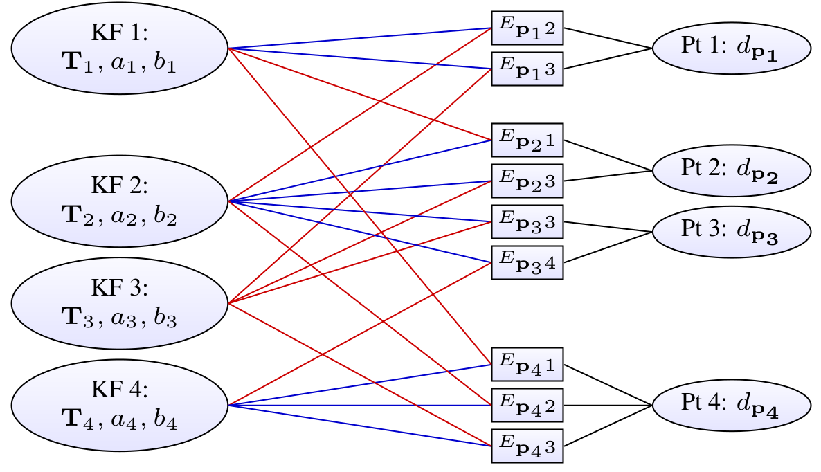
Example with four keyframes and four points; one in KF1, two in KF2, and one in KF4.

Each energy term depends on the point’s host frame (blue), the frame the point is observed in (red), and the point’s inverse depth (black). Further, all terms depend on the global camera intrinsics vector c, which is not shown.

Windowed Optimization

A total photometric error $E_{photo}$ in a sliding window is minimized using Gauss-Newton optimization.

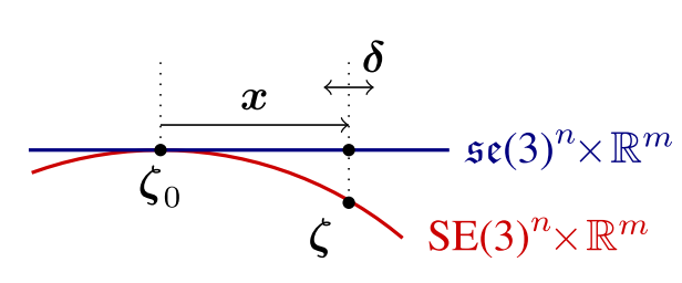
With Gauss-Newton step $\delta$, all optimized variables are denoted as $\zeta\in SE(3)^n\times \mathbb{R}^m$. Marginalizing a residual depending on $\zeta$ will fix the tangent space where delta updates  $x\in\mathfrak{se}(3)^n\times\mathbb{R}^m$ are accumulated. The evaluation point for this tangent space refers to $\zeta_0$. Therefore the current state estimate should be
$$
\zeta=x\boxplus\zeta_0
$$

Gauss-Newton Optimization

What is Gauss-Newton method?

Let linearized system be
$$
H\delta=b
$$
with
$$
H=J^TWJ\
b=-J^TWr
$$
where $\delta$ is perturbation. Here, $r\in \mathbb{R}^n$ is the residual vector and $J\in\mathbb{R}^{n\times d}$ is its Jacobian. $W\in\mathbb{R}^{n\times n}$ is diagonal weight matrix of residuals. The Hessian $H$ contains a LARGE diagonal block of correlations between the depth variables. By using Schur complement, inversion can be taken efficiently.

what is the dimensions of n, d

During optimization and marginalization, residuals are evaluated at $\zeta_0$, hence

$$ \begin{aligned} r_k&=r_k(x\boxplus \zeta_0) \\ &=(I_j[{\bf p}'({\bf T}_i,{\bf T}_j,d,{\bf c})]-b_j)-\frac{t_je^{a_j}}{t_ie^{a_i}}(I_i[{\bf p}-b_i]) \end{aligned} $$

and note that $$ x\boxplus \zeta_0:=({\bf T}_i, {\bf T}_j, d, {\bf c}, a_i, a_j, b_i, b_j) $$ Next, one single row in the Jacobian of pixel ${\bf p}_k$ in the neighborhood of ${\bf p}$ is given by $$ J_k=\frac{\partial r_k((\delta+x)\boxplus\zeta_0)}{\partial\delta} $$ Here note that $\boxplus$ means standard addition except for keyframe poses, where $\delta_p\boxplus T = e^{\delta_p}T$ as we defined. So now, we can decompose Jacobian as

$$ \begin{aligned} J_k&=[J_IJ_{geo},J_{photo}] \\ &=[\frac{\partial I_j}{\partial p_k'}\cdot \frac{\partial p'((\delta+x)\boxplus\zeta_o)}{\partial\delta_{geo}},\frac{\partial r_k((\delta+x)\boxplus\zeta_0)}{\partial\delta_{photo}} \end{aligned} $$

where $J_I$ is the image gradient and $\delta_{photo}$ corresponds to the photometric variables, $a_i, b_i, a_j, b_j$. The geometry Jacobian $J_{geo}$ contains derivatives of the pixel location, w.r.t. the geometric variables $T_i, T_j, d, c$. They are assumed to be the same as that of the central pixel for other neighbors.

Two approximations for real-time implementation

"First Estimate Jacobian" : $J_{photo}, J_{geo}$ are evaluated at $x=0$.

In Energy term, the absolute pose and scale are non-linear nullspaces. If we lost these nullspaces, the system will be unstable. Therefore Jacobians are evaluated at the SAME value, for variables they are connected to a marginalization factor. Because $J_{photo}, J_{geo}$ are smooth, so small increment of $x$ does not affect the null-spaces.

For further understanding of "First Estimate Jacobian", please refer to this paper.

Secondly, to reduce the computations, $J_{geo}$ is assumed to be the same for all residuals belonging to the same point, and evaluated only for the center pixel. (Authors insist they did not see significant differece when they applied this.)

Now, from the Gauss-Newton system, we can achieve an increment $\delta=H^{-1}b$ (which is in Lie algebra $\mathfrak{se}(3)$) and it is added to the current state:
$$
x^{new}\larr\delta+x
$$
Thanks to First Estimate Jacobian,
$$
J_k=\frac{\partial((\delta+x)\boxplus\zeta_0)}{\partial\delta}=\frac{\partial(\delta\boxplus(x\boxplus\zeta_0))}{\partial\delta}
$$
holds, therefore
$$
x^{new}\larr \log(\delta\boxplus e{^x})
$$
is equally valid.

• [x] Need to understand this update step... :(

Marginalization

When the active set of variables becomes too large, old variables are removed by marginalization using the Schur complement. Marginalize all points in $P_i$, as well as points that have not been observed in the last two keyframes.

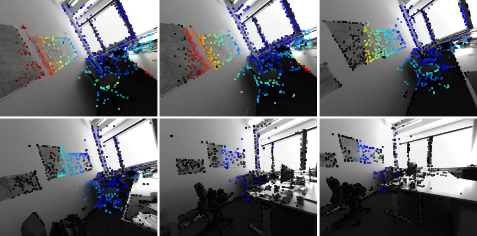
In the example above, colored points are diminishing and being turned black as they are marginalized. Observations of other points visible in the marginalized keyframe are dropped to maintain the sparsity structure of the Hessian.

$$ \begin{aligned} E&'(\zeta=x\boxplus \zeta_0)\\ &\approx 2(x-x_0)^T{\bf b}+(x-x_0)^T{\bf H}(x-x_0)+c\\ &=2x^T({\bf b}-{\bf H}x_0)+x^T{\bf H}x+(c+x_0^THx_0-x_0^T{\bf b})\\ &=2x^T{\bf b}'+x^T{\bf H}x+c' \end{aligned} $$

where $x_0$ denotes the current value of $x$ (evaluation point for $r$). Now it's a quadratic in $x$.

$$ \begin{bmatrix} {\bf H}_{\alpha\alpha} & {\bf H}_{\alpha\beta} \\ {\bf H}_{\beta\alpha} & {\bf H}_{\beta\beta} \end{bmatrix} \begin{bmatrix} {\bf x}_{\alpha} \\ {\bf x}_{\beta} \end{bmatrix} =\begin{bmatrix} {\bf b}'_{\alpha} \\ {\bf b}'_{\beta} \end{bmatrix} $$

$\alpha$ is the block of variables we want to keep, while $\beta$ is the block of variables we would like to marginalize. Now, Schur complement is applied to marginalize with $\hat{{\bf H}_{\alpha\alpha}}x_{\alpha}=\hat{{\bf b}'_{\alpha}}$ $$ \hat{{\bf H}_{\alpha\alpha}}={\bf H}_{\alpha\alpha}-{\bf H}_{\alpha\beta}{\bf H}_{\beta\beta}^{-1}{\bf H}_{\beta\alpha}\\ \hat{{\bf b}'_{\alpha}}={\bf b}'_{\alpha}-{\bf H}_{\alpha\beta}{\bf H}_{\beta\beta}^{-1}{\bf b}'_{\beta} $$ Therefore the residual energy on $x_\alpha$ can be written as $$ E'(x_\alpha\boxplus(\zeta_0)_\alpha)=2x^T_\alpha\hat{{\bf b}'_\alpha}+x^T_\alpha \hat{{\bf H}_{\alpha\alpha}} x_\alpha $$

This is a quadratic function on x and can be trivially added to the full photometric error Ephoto during all subsequent optimization and marginalization operations, replacing the corresponding non-linear terms. Note that this requires the tangent space for ζ0 to remain the same for all variables that appear in E? during all subsequent optimization and marginalization steps.

wtf..

Schur Complement

$$ M=\begin{bmatrix} A & B \\ C & D \end{bmatrix} $$

where $A, B, C, D$ are respectively $p\times p,\ p\times q,\ q\times p,\ q\times q$ , and $D$ is invertible. Then $$ \frac{M}{D}=A-BD^{-1}C \in \R^{p\times p}\\ \frac{M}{A}=D-CA^{-1}B \in \R^{q\times q} $$ are Schure complements of blocks $D, A$ in the matrix M.

VO Frontend

The frontend comprises of 3 parts:

• Finding sets $F, P_i$ and $obs({\bf p})$ for $E_{photo}$
• Initialization of parameters for $E_{photo}$
• Determining when a point/frame should be marginalized

Those are equivalent parts of keyframe detection, outlier removal, occlusion detection in indirect method.

Frame management

Authors kept a window with up to $N_f=7$ keyframes.

1. Initial Frame Tracking

• New keyframe created
• All active points are projected to new keyframe
• New incoming frames are tracked w.r.t this new keyframe. (multi-scale pyramid and constant motion model)

2. Keyframe Creation

Criteria for adding new keyframe

FoV changes - mean square optical flow
$$
f:=\big( \frac{1}{n}\sum_{i=1}^n | {\bf p}-{\bf p}' |^2 \big)^{\frac{1}{2}}
$$

Occlusion & disocclusion - mean flow without rotation
$$
f_t:=\big( \frac{1}{n}\sum_{i=1}^n | {\bf p}-{\bf p}_t' |^2 \big)^{\frac{1}{2}}
$$
where ${\bf p}'t$ with ${\bf R}={\bf I}{3\times 3}$

Camera exposure time change - relative brightness factor
$$
a:=|\log{(e^{a_j-a_i}t_jt_i^{-1})}|
$$

A keyframe is created if
$$
w_ff+w_{f_t}f_t+w_aa >T_{kf}
$$
where $w_f, w_{f_t}, w_a$ are respect wegiths and $T_{kf}=1$ by default.

3. Keyframe Marginalization

$I_1$ the latests, $I_n$ the oldest

The lastest two keyframes are kept

Frames with < 5% points in $I_1$ are marginalized

If # of frames are $>N_f$, the one maximizing distance score is marginalized
$$
s(I_i)=\sqrt{d(i,1)}\sum_{j\in[3,n]/{i}}(d(i,j)+\epsilon)^{-1}
$$
where $d(i,j)$ is the Euclidean distance between $I_i$ and $I_j$.

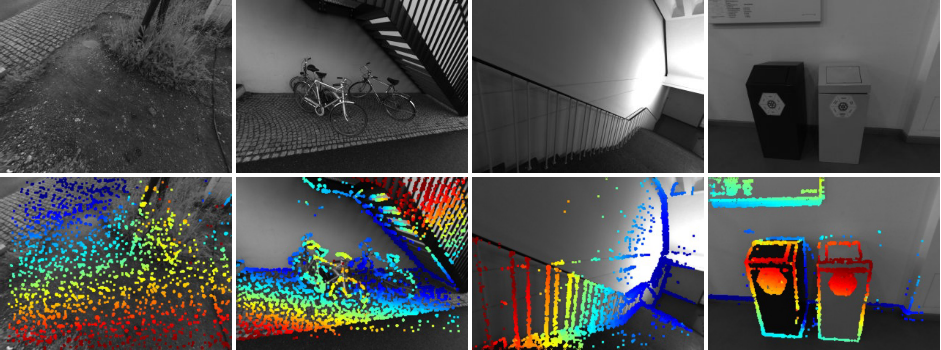
Point Management

The number of points are fixed as $N_p=2000$, all across the keyframes - equally distributed across space and active frames.

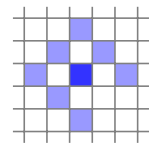
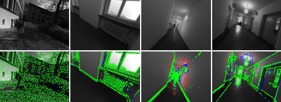
1. Candidate Point Selection

Reigion-adaptive threshold

• Split Image into blocks of 32X32
• compute $\bar{g}+g_{th}$, where $\bar{g}$ is median absolute gradient and $g_{th}=7$ a global constant

Point selection

• Split image into $d\times d$ blocks (d is also adaptive)
• Select a pixel with largest gradient with $g>g_{th}$
• If no pixels are included, repeat the process twice with block-size $2d$ and $4d$.
• This would capture weak-gradient points in smooth-plane such as white wall.

2. Candidate Point Tracking

Candidates are tracked, minimizing $E_{photo}$. From the best match, a depth and variance are calculated. They are used for constraining the search interval for next frame.

3. Candidate Point Activation

Candidates with largest distance from projected active points are chosen.

Outlier and Occlusion Detection

• Searching along epipolar line during candidate tracking, points for which the minimum is not sufficiently disntinct are discarded
• Points having photometric error surpassing the regional adaptive threshold $g$ are removed

Conclusion

Pros:

DSO can provide the state-of-the-art 3D point cloud, and still has the possibility to be improved by implementing IMU. Furthermore, in smooth-texture region, it shows supremeacy compared to other approaches.

Cons:

DSO has some compromisations to achieve real-time performance:

• Only 8 pixels are compared in a point
• Jacobians of residuals are approximated
• Linearization near $x$
• Having the same $J_{geo}$ across the pixels
• Keyframe creation by hand-tuned weights
• To make Hessian sparse, observations remaining in the frame are dropped.

Also suffering from iterations for optimization and marginalization. The framework is very complicated.

Reference

1. S. Leutenegger, S. Lynen, M. Bosse, R. Siegwart, and P. Fur- gale. Keyframe-based visual–inertial odometry using non- linear optimization. International Journal of Robotics Re- search, 34(3):314–334, 2015. 3, 6, 7, 13