[Review] VI-DSO (Eng)

Introduction

IMU measurement is accumulated and updated when new keyframe is added.

Dynamic marginalization - partial marginalization when scale is not accurate. Instead, some initial guess is used until scale become converged.

Remark

• a direct sparse visual-inertial odometry system.
• a novel initialization strategy where scale and gravity direction are included into the model and jointly opti- mized after initialization.
• we introduce ”dynamic marginalization” as a technique to adaptively employ marginalization strategies even in cases where certain variables undergo drastic changes.

Direct Sparse Visual-Inertial Odometry (VI-DSO)

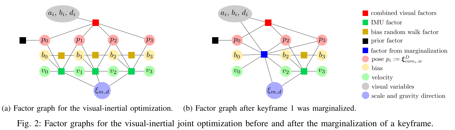
To make the problem computationally feasible the optimization is performed on a window of recent frames while all older frames get marginalized out.

The system runs two parallel loops:

• The coarse tracking is executed for every frame and uses direct image alignment combined with an inertial error term to estimate the pose of the most recent frame.
• When a new keyframe is created we perform a visual- inertial bundle adjustment like optimization that esti- mates the geometry and poses of all active keyframes.

Minimize:
$$
E_{total}=\lambda\cdot E_{photo}+E_{inertial}
$$

Inertial error

IMU preintegration allows adding a single IMU factor describing the pose between two camera frames. Inertial error is in form of normalized-squared sum.
$$
E_{inertial}(s_i,s_j):=(s_j\boxminus\hat{s}j)^T\hat{\Sigma}^{-1}{s,j}(s_j\boxminus\hat{s}_j)
$$
where the operator $\boxminus$ applies $\xi_j\boxplus(\hat{\xi_j})^{-1}$ for poses, and a normal subtraction for other components.

IMU Initialization and the problem of observability

Integration of IMU provides metric scale instead of relative camera scale, as well as gravity direction.

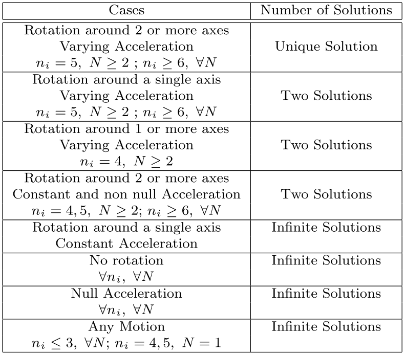
: Source: Martinelli, A. (2014). Closed-form solution of visual-inertial structure from motion. International Journal of Computer Vision, 106(2), 138–152. https://doi.org/10.1007/s11263-013-0647-7

For self-driving car, it is possible to have situations of

• Rotation around a single axis Varying Acceleration
• No rotation

In certain situation, immediate initialization could not be possible. The state-of-the-art SLAM cosumes first 15s for initialization.

In this paper, scale is initialized with arbitrary value. Initialization strategy is as following:

• Compute rough pose estimate between two frames and approximate depth for several points.
• Initial gravity direction is computed by averaging up to 40 acc. measurements.
• Initialize the velocity and IMU biases with zero and the scale with 1.0

All these parameters will be optimized.

SIM(3)-based Representation of the World

To incorporate scale and gravity direction into state vector, define DSO coordinate:
$$
T_{m_d} \in {T \in \text{SIM}(3)\ | \ \text{translation}(T) = 0}
$$
with corresponding
$$
\xi_{m_d}=log(T_{m_d})\in \mathfrak{sim}(3)
$$
Hence DSO coordinate is a scaled and rotated frame of the metric frame. Note that photometric error is evalutated in DSO frame, to be independent of scale and gravity, while inertial error is in metric frame.

Scale-aware Visual-Inertial Optimization

As IMU error between two subsequent keyframes increases, the time between the two is limited up to 0.5s. Optimized poses are represented in the DSO frame, so they do not depend on the scale.

Nonlinear optimization

Gauss-Newton algorithm is used. State vector is

$$ s_i:=[(\xi^D_{cam_{i\_w}})^T, v_i^T, b_i^T, a_i,b_i,d_i^1,d_i^2,\cdots,d_i^m]^T $$

where $v_i\in\mathbb{R}^3$ is the velocity, $b_i\in\mathbb{R}^6$ is the current IMU bias, $a_i, b_i$ are the affine illumination parameters, $d_i^j$ are the inverse depths of the points hosted in this keyframe. Therefore, the full state vector is defined as
$$
s=[C^T,\xi^T_{m_d},s^T_1,s^T_2,\cdots,s^T_n]^T
$$

where $c$ contains the geometric camera parameters and $\xi_{m_d}$ denotes the translation-free transformation between the DSO and the metric frame.

Now, using the stacked residual vector $r$ we have

$$ J=\dfrac{dr(s\boxplus\epsilon)}{d\epsilon}\bigg|_{\epsilon=0} \\\\\\ H=J^TWJ \\\\\\ b = -J^TWr $$

as we got Gauss-Newton system $\delta=H^{-1}b$.

Because there is no overapping residuals between $E_{photo}$ and $E_{inertial}$, we can divide $H, b$ as

$$ H=H_{photo}+H_{imu}\\\\\\ b=b_{photo}+b_{imu} $$

Recall that IMU is represented in the metric frame. So additional state vector is needed.

$$ s'_i:=[\xi^M_{w\_imu_i}, v_i, b_i]^T\\\\\\ s'=[s'^T_1,\cdots,s'^T_n]^T $$

The inertial residuals lead to

$$ H_{imu}'=J_{imu}'^T W_{imu}J_{imu}' \\\\\\ b'_{imu}=-J_{imu}'^T W_{imu} r_{imu} $$

For joint optimization,

$$ H_{imu}=J_{rel}^T H_{imu}'J_{rel} \\\\\\ b_{imu}=-J_{rel}^T b'_{imu} $$

Marginalization using the Schur-complement

Same as DSO.

Dynamic Marginalization for Delayed Scale Convergence

Marginalization priors

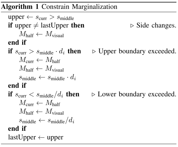
Maintaining priors $M_{visual}, \ M_{curr}, \ M_{half}$ and reset the one when the scale estimation is too far from the linearization point.

• $M_{curr}$ : used for state estimation from the moment that linearization point is set
• $M_{half}$ : contains only recent states
• $M_{visual}$ : scale independent information from previous states of vision

Priors visualization

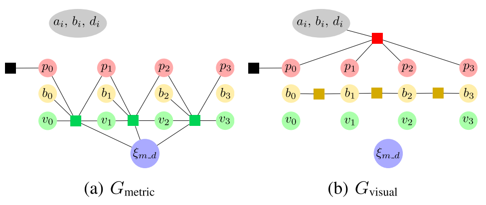
Define factor graph

$$
G_{full}=G_{metric}\cup G_{visual}
$$
$G_{metric}$ contains only visual-inertial factors (depending on $\xi_{m_d}$), and $G_{visual}$ contains all others.

For optimization, the graph is computed as
$$
G_{ba}=G_{metric}\cup G_{visual}\cup M_{curr}
$$
When keyframe $i$ is marginalized, $M_{visual}$ is updated with $G_{visual}\cup M_{visual}$.

Scale estimates

$s_i:=$ scale estimate at the time, $i$ was marginalized. $i\in M$ iff $M$ contains inertial factor. This leads to this constraint:
$$
\forall i \in M_{curr}:s_i\in [s_{middle}/d_i, s_{middle}\cdot d_i]
$$

$$
\forall i\in M_{half}:s_i \in \left{
\begin{eqnarray}
[s_{middle}, s_{middle}\cdot d_i], & \text{if} \ s_{curr} > s_{middle} \
[s_{middle}/d_i, s_{middle}], & \text{otherwise}
\end{eqnarray}
\right.
$$

In order to preserve those constraints, below algorithm must be applied everytime when marginalization happens.

Coarse Visual-Inertial Tracking

Fast computation of pose estimation for each frame

IMU preintegration is used between keyframe ~ current frame

After Joint optimization is finished, the coarse tracking is re-initialized.

Conclusion

Pros:

• The system can estimate scale and gravity direction.

• Improved precision and accuracy by using IMU, compared to original DSO
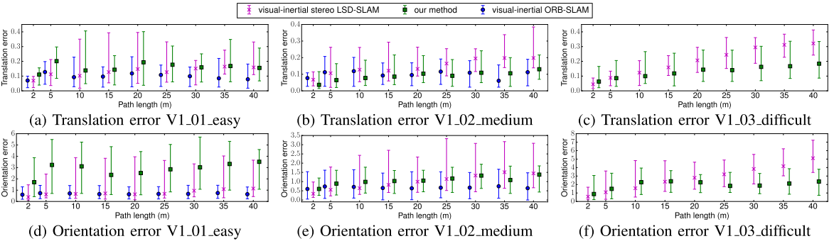
• In presence of extreme dynamic, VI-DSO shows robust result, but in little-to-moderate conditions, it does not have significant improvements compared to LSD-SLAM and ORB-SLAM.

Cons:

• Scale is not clearly observable, hence initial guess is needed. This induces dynamic marginalization.
• For certain situations, initial states cannot be initialized properly (previous studies spends 15 ~ 30 seconds for this initialization).